Radar Measurements of Two Vehicles with Three Cooperative Imaging Sensors
- Citation Author(s):
- Submitted by:
- Johannes Schlichenmaier
- Last updated:
- DOI:
- 10.21227/wwt7-w739
- Data Format:
- Research Article Link:
 1344 views
- Categories:
- Keywords:
Abstract
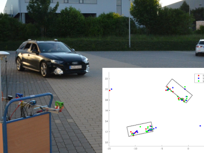
Presented are the target lists of a total of 8718 measurement frames produced by three (3) radar sensors, matched together with the IMU+GNSS-RTK solution for position and motion of two (2) automobiles. The sensors are synced in respect to their measurement times, but operate independently. Their modulation is offset by a certain frequency, to ensure mono-static evaluation. This allows for a cooperative evaluation of measurements. The sensor positions are static. The two automobiles are driving maneuvers in front of the three radar sensors, including following, overtaking, driving alongside, and driving towards each other. The data set is available in three different CFAR threshold variants. Included is a description of the setup and radar modulation parameters, the data structure, as well as a minimum working example of how to work with the data.
Instructions:
The data is provided in the form of MAT files containing simple data types and tables (supported by
MATLAB versions >= 2013b).
The following code example loads the data from a single MAT file and plots a full set of measurement
frames at around 8 Hz. For a full documentation, please refer to the uploaded README files.
It is important to remember, that the target lists include all target points, whether or not they
are a peak point. Only in combination of the sensor and frame specific peak IDs, the peak values can
be extracted.
% load measurement file
tl_content = load(['cfar_10_12_pe' filesep '20200624_Car2_Kreise_1.mat']);

% prepare figure
hfig = figure();
haxes = axes(hfig);

plot_tl_s5 = scatter(nan,nan, 'r', 'filled');
hold(haxes, 'on');
plot_tl_s7 = scatter(nan,nan, 'b', 'filled');
plot_tl_s8 = scatter(nan,nan, 'g', 'filled');

plot_gt_1 = plot(nan, nan, 'k', 'LineWidth', 1.5);
plot_gt_2 = plot(nan, nan, 'k', 'LineWidth', 1.5);
hold(haxes, 'off');

haxes.DataAspectRatio = [1,1,1];
xlim(haxes, [-50,50]);
ylim(haxes, [0,50]);

% plot measurement
num_frames = size(tl_content.data,1);

for i_frame = 1:num_frames
    % plot peak target points of sensor 5
    peak_ids_s5 = tl_content.data.te_peak_ids{i_frame,5};
    plot_tl_s5.XData = tl_content.data.target_list{i_frame,5}.x(peak_ids_s5);
    plot_tl_s5.YData = tl_content.data.target_list{i_frame,5}.y(peak_ids_s5);

    % plot peak target points of sensor 7
    peak_ids_s7 = tl_content.data.te_peak_ids{i_frame,7};
    plot_tl_s7.XData = tl_content.data.target_list{i_frame,7}.x(peak_ids_s7);
    plot_tl_s7.YData = tl_content.data.target_list{i_frame,7}.y(peak_ids_s7);

    % plot peak target points of sensor 8
    peak_ids_s8 = tl_content.data.te_peak_ids{i_frame,8};
    plot_tl_s8.XData = tl_content.data.target_list{i_frame,8}.x(peak_ids_s8);
    plot_tl_s8.YData = tl_content.data.target_list{i_frame,8}.y(peak_ids_s8);

    % plot ground truth OBB of object 1
    gt_1_points = [tl_content.data.ground_truth{i_frame}.polyshape(1).Vertices;
        tl_content.data.ground_truth{i_frame}.polyshape(1).Vertices(1,:)];
    plot_gt_1.XData = gt_1_points(:,1);
    plot_gt_1.YData = gt_1_points(:,2);

    % plot ground truth OBB of object 2
    gt_2_points = [tl_content.data.ground_truth{i_frame}.polyshape(2).Vertices;
        tl_content.data.ground_truth{i_frame}.polyshape(2).Vertices(1,:)];
    plot_gt_2.XData = gt_2_points(:,1);
    plot_gt_2.YData = gt_2_points(:,2);

    pause(0.1);
end


